Just like with straight lines, the topic of quadratics (or quadratic functions, or parabolas – all these terms mean the same thing), ultimately boils down to a single equation – the General Equation of a Quadratic Function:

Unlike with straight lines, where the constants m and c (the gradient and y-intercept respectively) had names, the coefficients a, b and c don’t have separate names (unhelpfully…)

x and y are simply coordinates on typical x–y axes, and given that they are variables, x and y will change depending on the position you’re looking at on a quadratic graph. However, for any specific quadratic function, the coefficients \boldsymbol{a}, \boldsymbol{b} and \boldsymbol{c} are fixed.

As you no doubt already know, quadratics are not straight lines – they are curved lines with a line of symmetry through their turning point. As an example, the quadratic y=x^{2}-6x+8 is shown below:

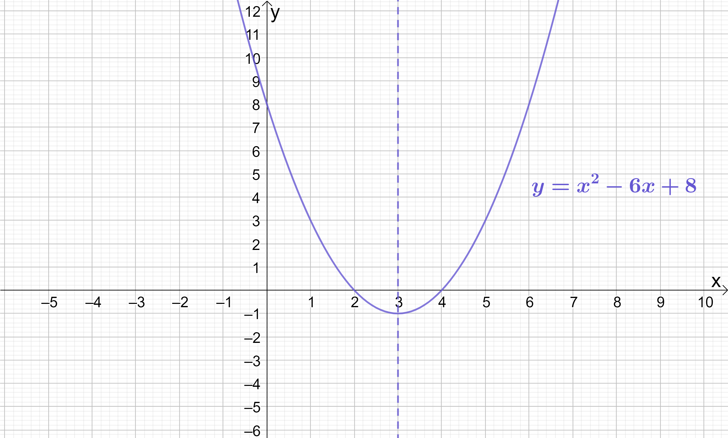
But why are they curved? What is it about quadratics that makes them curved instead of straight?

It’s all because of the x^{2} term. In straight lines, which can all be written in the form of the General Equation y=mx+c, there is no powered x term. Once you start introducing x terms with powers such as x^{2}, x^{3}, x^{4} and so on, the behaviour of graphs changes drastically and they become much more complicated than simple straight lines.

Let’s compare the simplest straight line, y=x (which we met in the previous chapter), with the simplest quadratic, y=x^{2}, to understand how quadratics end up being curved instead of straight.

We can sketch both functions using a very basic coordinate table method. We can create coordinate tables by substituting different values of x into each function to calculate the corresponding values of y and then plot the results as coordinates in the form (x, y). Here it is useful to look at both positive and negative values of x for both functions:

1) Choose some x values: -3, -2, -1, 0, 1, 2, 3

2) Substitute these values into the equation to calculate corresponding y values:

\begin{aligned}y&=x \\[12pt]y&=(-3)=-3 \\[12pt]y&=(-2)=-2 \\[12pt]y&=(-1)=-1 \\[12pt]y&=(0)=0 \\[12pt]y&=(1)=1 \\[12pt]y&=(2)=2 \\[12pt]y&=(3)=3\end{aligned}

3) Summarise results in a coordinate table:

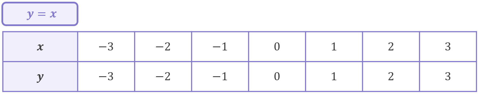
4) Plot the points on x–y coordinate axes:

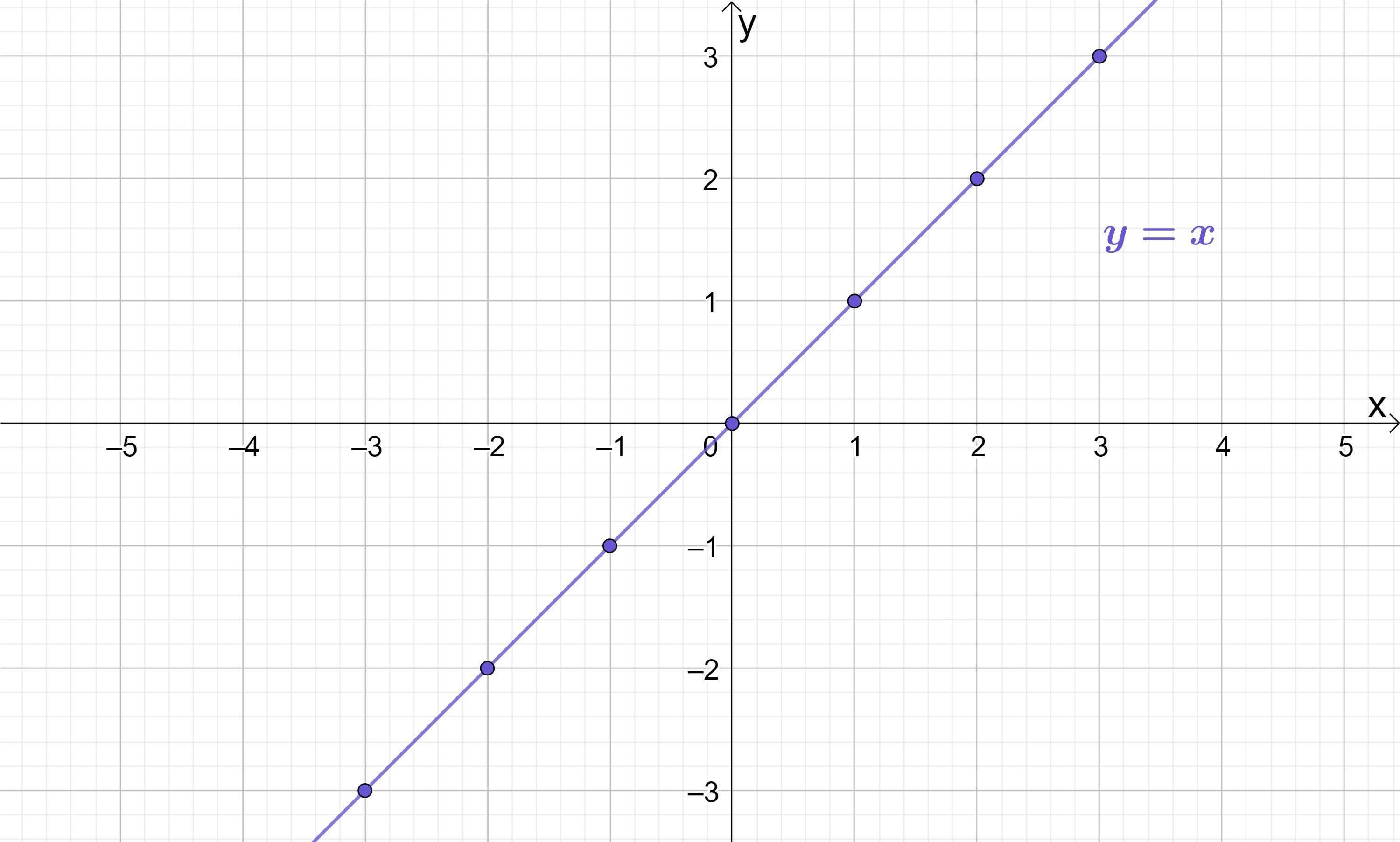
There should be nothing surprising about this graph at this stage – it is a simple straight line with all equal coordinates, a gradient of 1 and a y-intercept of (0, 0).

Notice that because the gradient is 1, every time x increases or decreases by 1 then y also increases or decreases by 1:

Repeating this process with the simplest quadratic function y=x^{2}, we have the following:

1) Choose some x values: -3, -2, -1, 0, 1, 2, 3

2) Substitute these values into the equation to calculate corresponding y values:

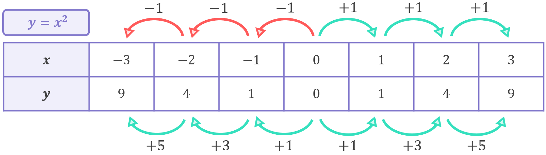
\begin{aligned}y&=x^{2} \\[12pt]y&=(-3)^{2}=9 \\[12pt]y&=(-2)^{2}=4 \\[12pt]y&=(-1)^{2}=1 \\[12pt]y&=(0)^{2}=0 \\[12pt]y&=(1)^{2}=1 \\[12pt]y&=(2)^{2}=4 \\[12pt]y&=(3)^{2}=9\end{aligned}

3) Summarise results in a coordinate table:

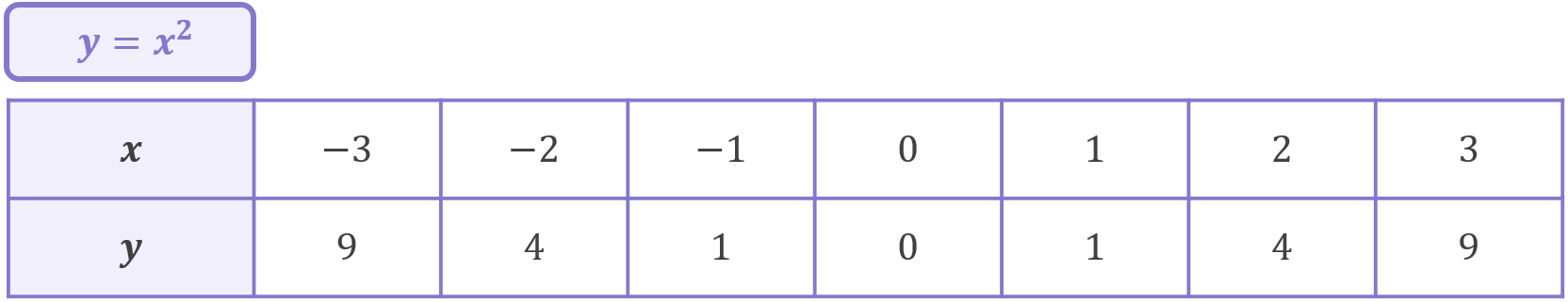
4) Plot the points on x–y coordinate axes:

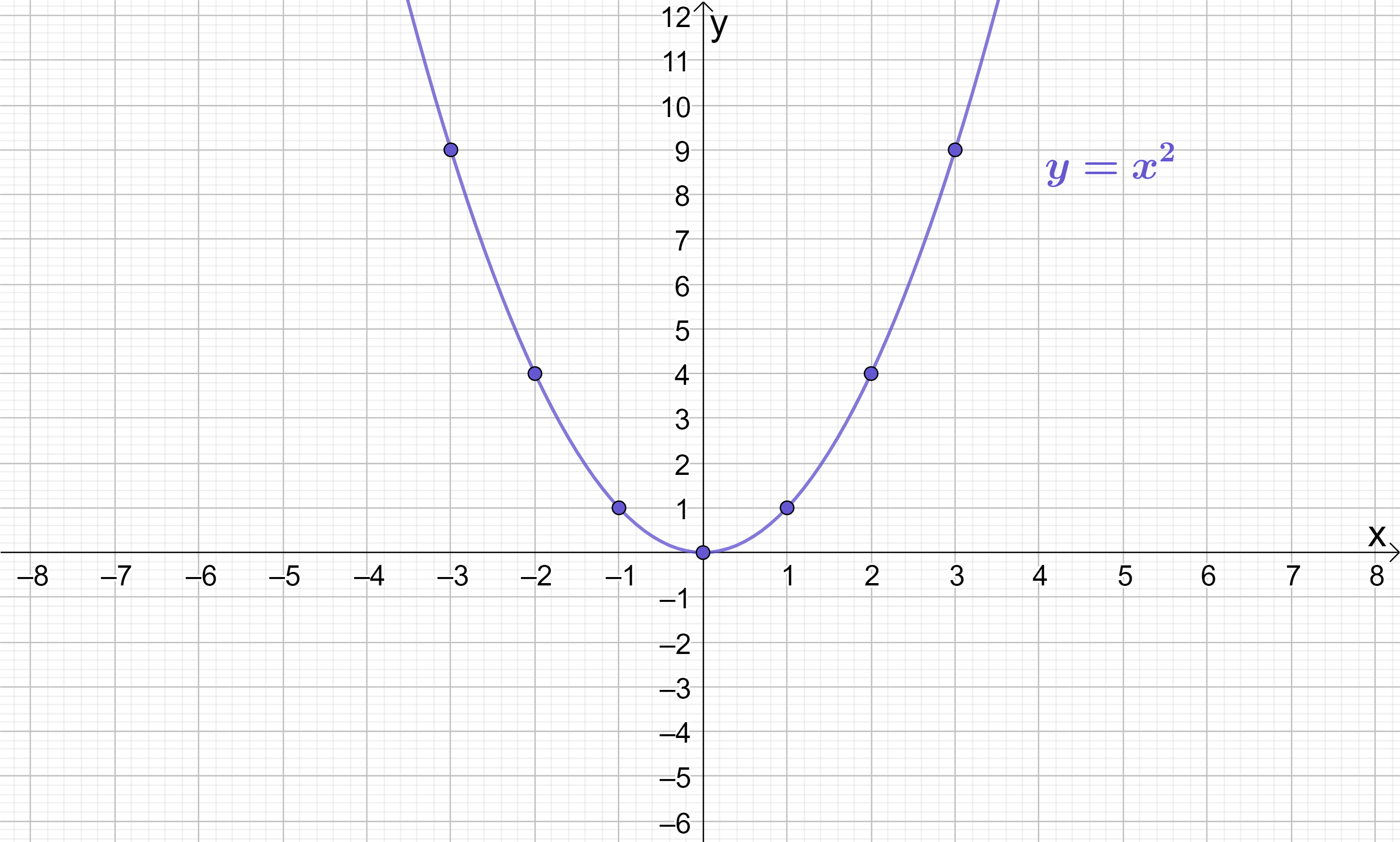
This graph shows some very different behaviour, and it is quite clearly non-linear. Since any number squared is always positive, there are no negative y values even when x is negative, which results in a line of symmetry running through the turning point. In this case, the turning point is the coordinate (0, 0) and the line of symmetry is the y-axis itself.

If someone asked you what the gradient of this quadratic is, what would you say? That’s sort of a confusing question isn’t it? Because, unlike straight lines which have an obvious slope which does not change, a quadratic is sloped differently at different points. At some points the graph is very steep, whilst at others the graph flattens out. Because of this, when x increases or decreases by 1, then y does not always increase or decrease by an equivalent amount.

This is what causes the graph to become curved. Looking again at the coordinate table for y=x^{2} and starting from the x=0 position, we can see that for every jump of 1 in x, y does not always move by the same amount:

What this exercise shows is that including an x^{2} term in a function causes it to become a symmetric curve. The \boldsymbol{x^{2}} term is what gives the quadratic its characteristic symmetrically curved shape. If there’s no \boldsymbol{x^{2}} term, then a function cannot be a quadratic.

The quadratic we examined above, y=x^{2}, is the simplest quadratic function. Although it may not look like it at first, this quadratic is in fact in the form of the General Equation y=ax^{2}+bx+c. If we write our quadratic y=x^{2} in a more expanded form, this becomes clearer:

\begin{aligned}y&=x^{2} \\[12pt]y&=1x^{2}+0x+0\end{aligned}

Do the changes I have made actually do anything? No, they don’t – these two lines say exactly the same thing! Explicitly showing a coefficient of 1 before the x^{2} term doesn’t do anything since multiplying by 1 has no effect, and any term with a 0 attached to it will just disappear since multiplying by 0 always gives 0. However, comparing this to the General Equation it is now clearer that our original quadratic is in fact in standard form:

\begin{aligned}y&=x^{2} \\[12pt]y&=1x^{2}+0x+0 \\[12pt]y&=ax^{2}+bx+c\end{aligned}

The simplest quadratic, y=x^{2}, therefore has coefficients a=1, b=0 and c=0.

If we were to change the \boldsymbol{a}, \boldsymbol{b} and \boldsymbol{c} coefficients of \boldsymbol{y=x^{2}} or any other quadratic function, the function’s curvature and position will be affected. 

Compare the graph of the simplest quadratic, y=x^{2}, which has coefficients a=1, b=0 and c=0, to the graph of another random quadratic, say y=4x^{2}-12x+10, which has coefficients a=4, b=-8 and c=6, and you can see there are clear differences in the curvature (or steepness) and position of the two graphs:

All quadratics have 4 key features:

1) Nature
2) \boldsymbol{y}-intercept
3) \boldsymbol{x}-intercepts (or “roots”); and
4) Turning point

These 4 features are highlighted on the quadratic y=x^{2}-4x+3 shown below:

In the following topics, we will explore how the a, b and c coefficients of a quadratic impact these 4 features.